How-to: Generate Quasi-Vertical Profiles.

Daniel Sanchez-Rivas¹ and Miguel A. Rico-Ramirez¹

¹Department of Civil Engineering, University of Bristol, Bristol, BS8 1TR, United Kingdom

This notebook describes the process of retrieving, quality-check and processing raw C-band radar data collected by the operational UK Met Office radar network.

UK Met Office C-band rain radar dual-polarisation products are available at http://catalogue.ceda.ac.uk/uuid/82adec1f896af6169112d09cc1174499 (Met Office, 2003)

Import relevant packages

import towerpy as tp
import cartopy.crs as ccrs

# %matplotlib notebook

---------------------------------------------------------------------------
ModuleNotFoundError                       Traceback (most recent call last)
Cell In[1], line 1
----> 1 import towerpy as tp
      2 import cartopy.crs as ccrs
      4 # %matplotlib notebook

ModuleNotFoundError: No module named 'towerpy'

Define working directory and file name

For this example, we’ll use data collected at the Chenies radar site; In the file name, augzdr stands for polarimetric data, sp for short-pulse and el4 refers to collected at 9.0° elevation angle.

RSITE = 'chenies'
WDIR = f'../../../datasets/ukmo-nimrod/data/single-site/2020/{RSITE}/spel4/'
FNAME = (f'metoffice-c-band-rain-radar_{RSITE}_202010030730_raw-dual-polar-'
         + 'augzdr-sp-el4.dat')

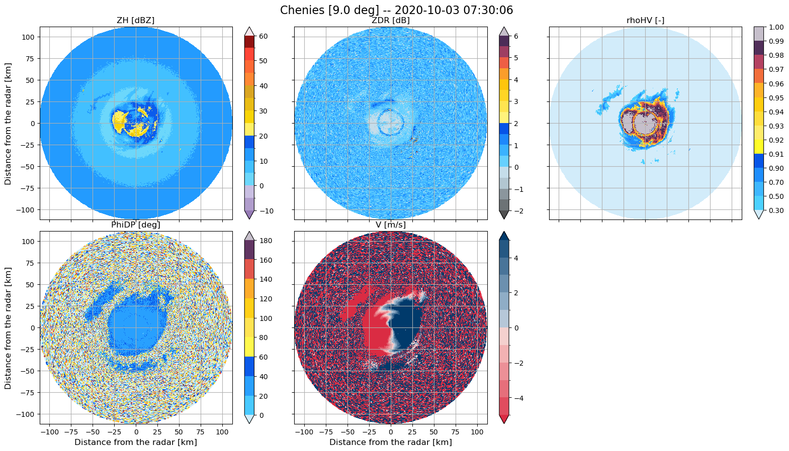
Use Towerpy to read in the raw radar variables.

The Rad_scan class initialises a radar object.

Within the ukmo module, the ppi_ukmoraw function provides an interface to read the current binary format used by the MO to store the radar data.

Note that the argument exclude_vars was used to discard the ‘W [m/s]’, ‘SQI [-]’ and ‘CI [dB]’] variables, as they will not be used at this stage.

rdata = tp.io.ukmo.Rad_scan(WDIR+FNAME, RSITE)
rdata.ppi_ukmoraw(exclude_vars=['W [m/s]', 'SQI [-]', 'CI [dB]'])
rdata.ppi_ukmogeoref()

#tp.datavis.rad_display.plot_ppi(rdata.georef, rdata.params, rdata.vars)
tp.datavis.rad_display.plot_setppi(rdata.georef, rdata.params, rdata.vars)

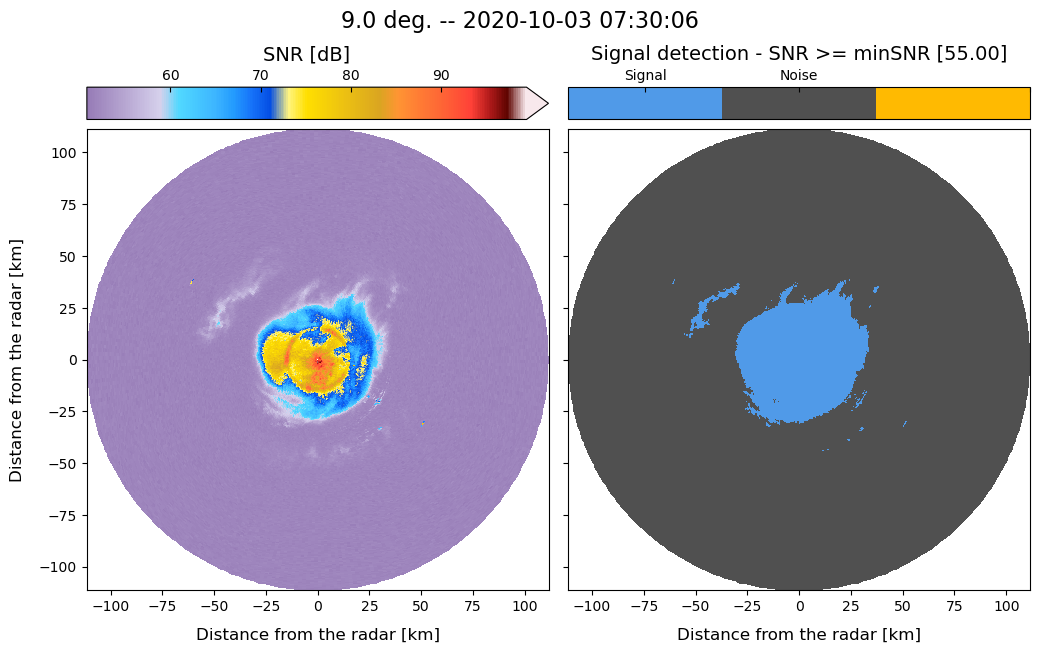
Computation of the Signal-to-Noise-Ratio

We use the signalnoiseratio function to compute the Signal-to-Noise-Ratio (SNR) (in dB) and discard data using a reference noise value equal to 55 dB. This value had been checked at all the UK Met office radar sites (valid only for short-pulse scans) and proved effective in removing noise within the scans.

The data2correct argument copies the original data and generates a new dictionary containing radar variables but SNR filtered.

rsnr = tp.eclass.snr.SNR_Classif(rdata)
rsnr.signalnoiseratio(rdata.georef, rdata.params, rdata.vars, min_snr=55,
                      data2correct=rdata.vars, plot_method=True)

Generation of QVPs of polarimetric variables

We use the pol_qvps function to generate quasi-vertical profiles of polarimetric variables.

Note that the argument stats is set to True to compute statistics related to the averaging process of the rays to enable a comprehensive analysis of the profiles.

rprofs = tp.profs.polprofs.PolarimetricProfiles(rdata)
rprofs.pol_qvps(rdata.georef, rdata.params, rsnr.vars, stats=True)

Use the plot_radprofiles function to view the QVPs.

tp.datavis.rad_display.plot_radprofiles(rprofs,
                                        rprofs.georef['profiles_height [km]'],
                                        colours=True)

<Figure size 640x480 with 0 Axes>

ML detection

Then we will run the method proposed by Sanchez-Rivas, D. and Rico-Ramirez, M. A. (2021) to detect the boundaries of the ML within the QVPs.

In the ml_detection function, we set a minimum height for the algorithm to search the ML signatures. The user can modify this and other arguments to fine-tune the algorithm’s performance.

Note that the plot_method argument is set to True. This argument displays an interactive plot that illustrates the steps followed by the ML detection algorithm. As the method computes all the possible combinations of the normalised profiles, it is possible to check each one by moving the slider.

rmlyr = tp.ml.mlyr.MeltingLayer(rprofs)
rmlyr.ml_detection(rprofs, min_h=0.25, comb_id=14, plot_method=True)

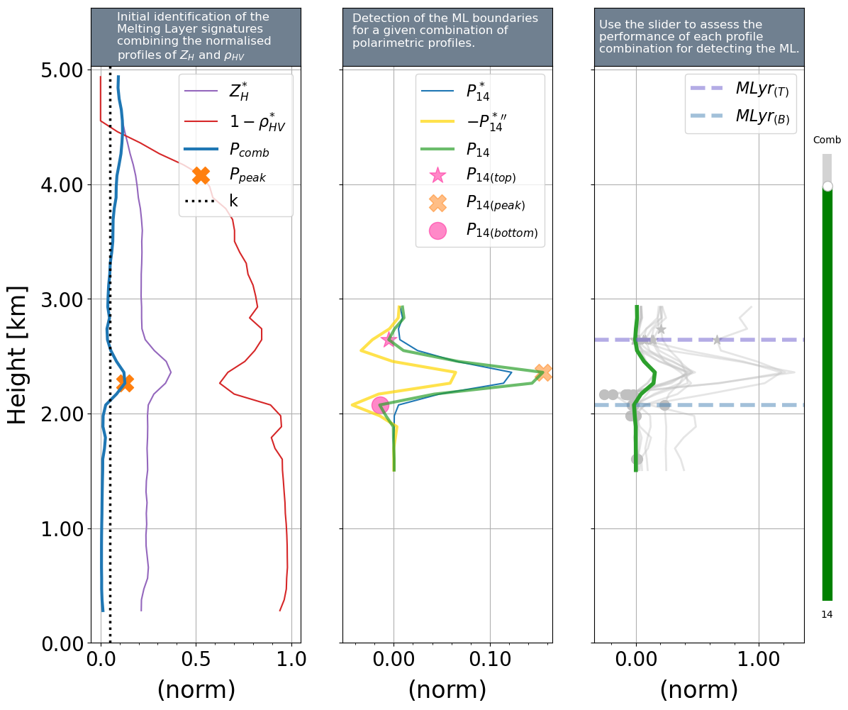
rmlyr.ml_top

np.float64(2.6442825147678377)

rmlyr.ml_thickness

np.float64(0.569356063449959)

rmlyr.ml_bottom

np.float64(2.0749264513178787)

These value are (much) the same to those obtained using VPs

$Z_{DR}$ offset detection

The offsetdetection_qvps function adapts the method proposed by Sanchez-Rivas, D. and Rico-Ramirez, M. A. (2022) to detect the $Z_{DR}$ offset using QVPs.

The mlyr is required to separate between liquid and solid precipitation. Whereas the min_h and other arguments help adjust the algorithm’s performance.

According to this method, the intrinsic value of $Z_{DR}$ in light rain at ground level is required. The default for this radar is 0.182. See the paper for a more detailed description.

rcalzdr = tp.calib.calib_zdr.ZDR_Calibration(rdata)
rcalzdr.offsetdetection_qvps(pol_profs=rprofs, mlyr=rmlyr, min_h=0.25, zdr_0=0.182)

rcalzdr.zdr_offset

np.float64(-0.2755357495838535)

This value is (much) the same to the one obtained from the method based in birdbath scans

References

Met Office (2003): Met Office Rain Radar Data from the NIMROD System. NCAS British Atmospheric Data Centre, 2022. http://catalogue.ceda.ac.uk/uuid/82adec1f896af6169112d09cc1174499

Sanchez-Rivas, D. and Rico-Ramirez, M. A. (2021), “Detection of the melting level with polarimetric weather radar” in Atmospheric Measurement Techniques Journal, Volume 14, issue 4, pp. 2873–2890, 13 Apr 2021 https://doi.org/10.5194/amt-14-2873-2021

Sanchez-Rivas, D. and Rico-Ramirez, M. A. (2022): “Calibration of radar differential reflectivity using quasi-vertical profiles”, Atmos. Meas. Tech., 15, 503–520, https://doi.org/10.5194/amt-15-503-2022