
How-to: Read-in, process and display UK Met Office radar data.#
Daniel Sanchez-Rivas1 and Miguel A. Rico-Ramirez1
1Department of Civil Engineering, University of Bristol, Bristol, BS8 1TR, United Kingdom
This notebook describes the process of retrieving, quality-check and processing raw C-band radar data collected by the operational UK Met Office radar network.#
UK Met Office C-band rain radar dual-polarisation products are available at http://catalogue.ceda.ac.uk/uuid/82adec1f896af6169112d09cc1174499 (Met Office, 2003)
Import relevant packages#
Users can also check the Python script (*.py) version of this processing steps here
import numpy as np
import towerpy as tp
import cartopy.crs as ccrs

# %matplotlib notebook
---------------------------------------------------------------------------
ModuleNotFoundError                       Traceback (most recent call last)
Cell In[1], line 1
----> 1 import numpy as np
      2 import towerpy as tp
      3 import cartopy.crs as ccrs

ModuleNotFoundError: No module named 'numpy'
Define working directory and file name#
For this example, we’ll use data collected at the Chenies radar site; augzdr stands for polarimetric data, lp for long-pulse and el0 refers to collected at 0.5° elevation angle.
RSITE = 'chenies'
WDIR = f'../../../datasets/ukmo-nimrod/data/single-site/2020/{RSITE}/lpel0/'
FNAME = (f'metoffice-c-band-rain-radar_{RSITE}_202010030729_raw-dual-polar-'
         + 'augzdr-lp-el0.dat')
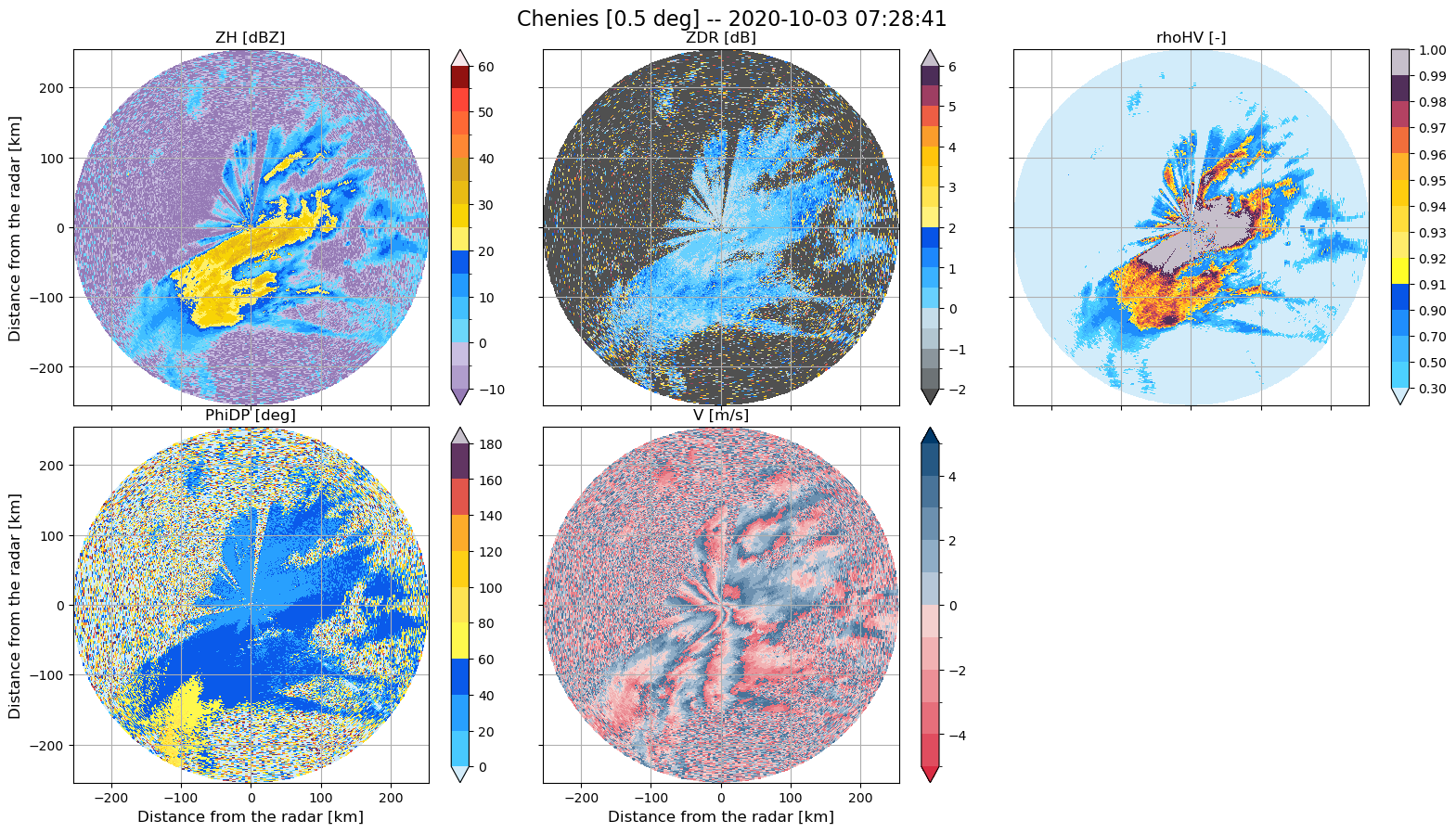
Use of Towerpy to read in the raw radar variables.#
The Rad_scan class initialises a radar object.
Within the ukmo module, the ppi_ukmoraw function provides an interface to read the current binary format used by the MO to store the radar data.
Note that the argument exclude_vars was used to discard the ‘W [m/s]’, ‘SQI [-]’ and ‘CI [dB]’] variables, as they will not be used at this stage.
rdata = tp.io.ukmo.Rad_scan(WDIR+FNAME, RSITE)
rdata.ppi_ukmoraw(exclude_vars=['W [m/s]', 'SQI [-]', 'CI [dB]'])
rdata.ppi_ukmogeoref()

# Plot all the radar variables
tp.datavis.rad_display.plot_setppi(rdata.georef, rdata.params, rdata.vars)
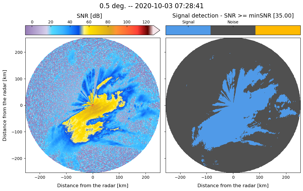
Computation of the Signal-to-Noise-Ratio#
We use the signalnoiseratio function to compute the Signal-to-Noise-Ratio (SNR) (in dB) and discard data using a reference noise value equal to 35 dB. This value had been checked at all the UK Met office radar sites (valid only for long-pulse scans) and proved effective in removing noise within the scans.
The data2correct argument copies the original data and generates a new dictionary containing radar variables but SNR filtered.
rsnr = tp.eclass.snr.SNR_Classif(rdata)
min_snr = 35
rsnr.signalnoiseratio(rdata.georef, rdata.params, rdata.vars, min_snr=min_snr,
                      data2correct=rdata.vars, plot_method=True)
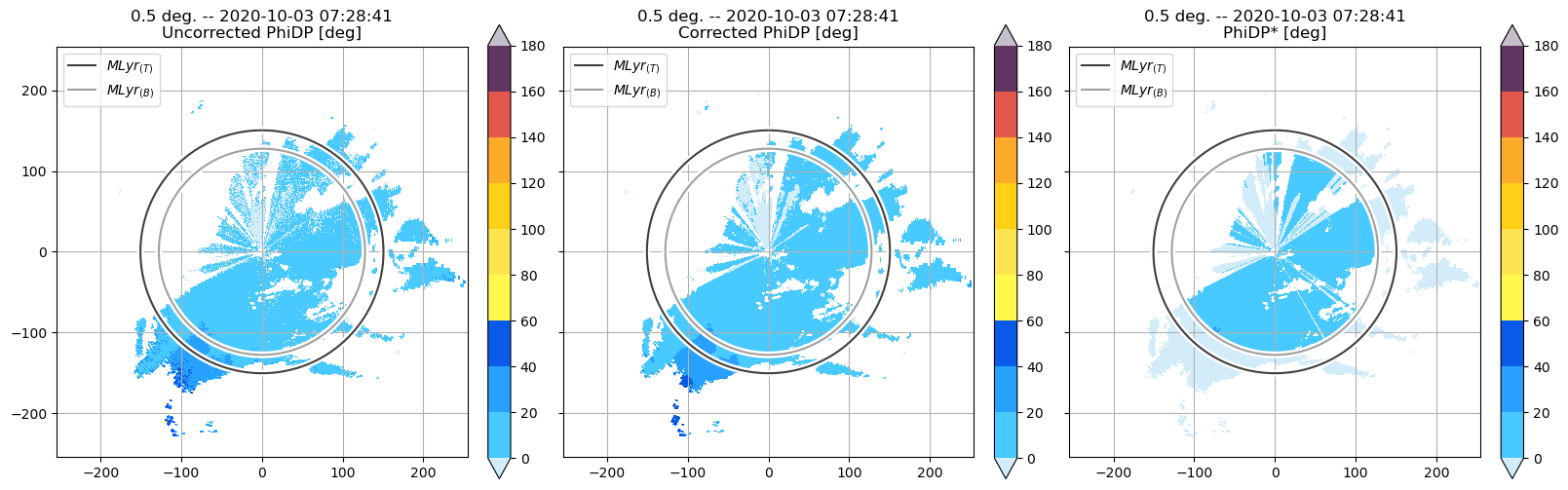
PhiDP offset correction#
There is a function implemented in Towerpy for estimating $\Phi_{DP}(0)$. Note that the output is similar to that obtained from VPs (40 deg).
ropdp = tp.calib.calib_phidp.PhiDP_Calibration(rdata)
ropdp.offsetdetection_ppi(rsnr.vars)
print(f'Phi_DP(0) = {ropdp.phidp_offset:.2f}')

ropdp.offset_correction(rsnr.vars['PhiDP [deg]'],
                        phidp_offset=ropdp.phidp_offset,
                        data2correct=rsnr.vars)
Phi_DP(0) = 36.65
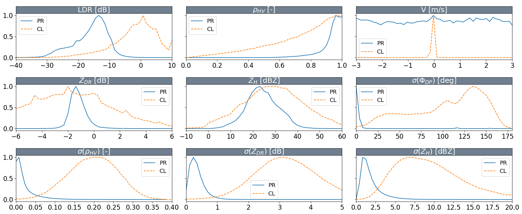
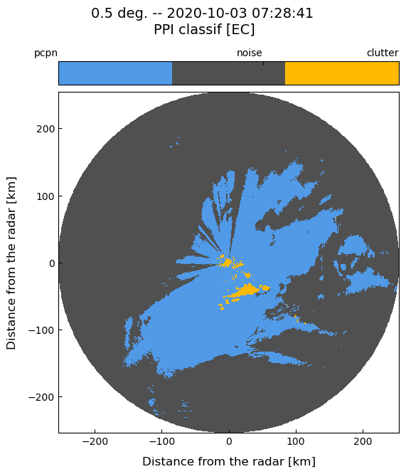
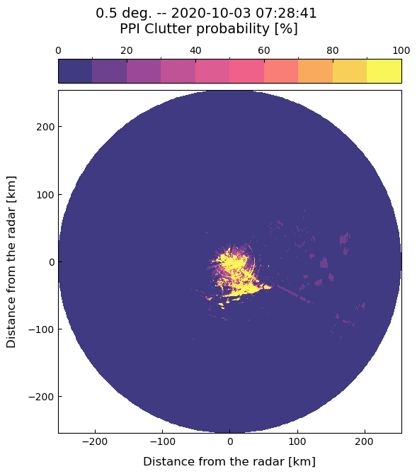
Classification of non-meteorological echoes#
Towerpy provides membership functions (MFS) to detect clutter echoes. These MFS were calibrated using C-band radar data. We plot the MFS using the plot_mfs function.
Note that the textures of polarimetric variables are a great clutter/meteorological echo discriminators!
tp.datavis.rad_display.plot_mfs(f'../../../towerpy/eclass/mfs_cband/')
We use the clutter_id function to identify clutter echoes. This function is based on the methodology proposed by Rico-Ramirez, M. A., & Cluckie, I. D. (2008).
This function requires descriptors of the azimuth, gates and other georeferenced data (rdata.georef); radar technical details (rdata.params); radar variables (rdata.vars), and other arguments that can be customised by the user.
As we’re working with Chenies radar data taken at 0.5 elevation angle, we load the array that contains the corresponding clutter map.
As above, The data2correct argument copies given data and generates a new dictionary containing radar variables but with the clutter echoes removed.
clmap = f'../../../towerpy/eclass/ukmo_cmaps/{RSITE}/chenies_cluttermap_el0.dat'

rnme = tp.eclass.nme.NME_ID(rsnr)
rnme.clutter_id(rdata.georef, rdata.params, ropdp.vars, binary_class=223,
                min_snr=rsnr.min_snr, clmap=np.loadtxt(clmap),
                data2correct=ropdp.vars, plot_method=True)
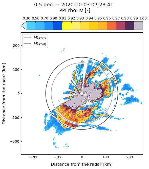
Definition of the melting layer boundaries#
We create a MeltingLayer object to set the melting level height and the melting layer thickness. These heights are important to delimit the rain region within the PPI scan. For this step, we estimated the melting layer boundaries from QVPs, but assuming an isotropic melting layer.
We can use the ml_ppidelimitation function to create a PPI depicting the limits of the melting layer.
rmlyr = tp.ml.mlyr.MeltingLayer(rdata)
rmlyr.ml_top = 2.64
rmlyr.ml_thickness = 0.57
rmlyr.ml_bottom = 2.08

rmlyr.ml_ppidelimitation(rdata.georef, rdata.params, rsnr.vars)

# Plot rhoHV and the ML
tp.datavis.rad_display.plot_ppi(rdata.georef, rdata.params, rnme.vars, var2plot='rhoHV [-]', mlyr=rmlyr)
Calibration of $Z_{DR}$#
We create a ZDR_Calibration object to define and correct the $Z_{DR}$. For this example, the $Z_{DR}$ offset is set as -0.27. This value was derived from QVPs and corroborated with birdbath scans.
rozdr = tp.calib.calib_zdr.ZDR_Calibration(rdata)
rozdr.offset_correction(rnme.vars['ZDR [dB]'],
                        zdr_offset=-0.27,
                        data2correct=rnme.vars)
Attenuation correction#
The next step is to correct the attenuation of the radar signal. We use the algorithms proposed by Bringi, V. N. et al (2001) and Rico-Ramirez, M. A. (2012).
The AttenuationCorrection object contains two functions, zh_correction and zdr_correction that correct the attenuation on $Z_H$ and $Z_{DR}$, respectively.
Note that the attenuation is computed up to a user-defined height that correspond to the rain region within the PPI scan.
rattc = tp.attc.attc_zhzdr.AttenuationCorrection(rdata)
rattc.zh_correction(rdata.georef, rdata.params, rozdr.vars,
                    rnme.nme_classif['classif [EC]'], attc_method='ABRI',
                    mlyr=rmlyr, pdp_pxavr_azm=3, pdp_dmin=1,
                    pdp_pxavr_rng=round(4000/rdata.params['gateres [m]']),
                    plot_method=True)
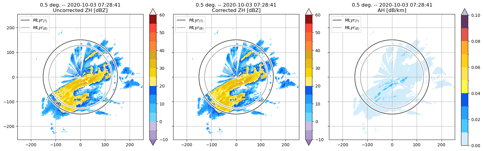
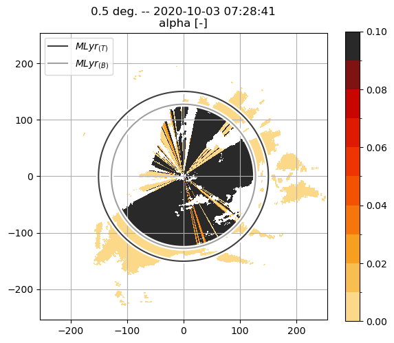
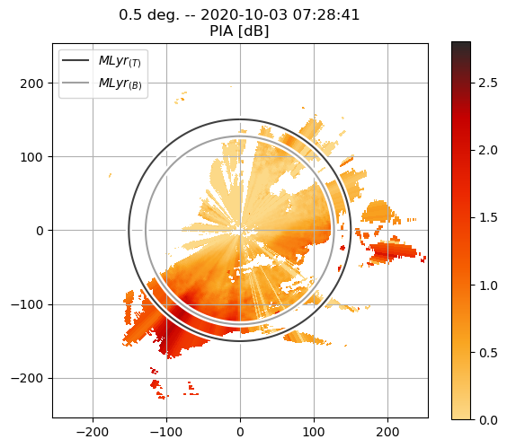
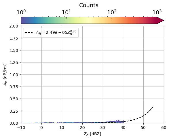
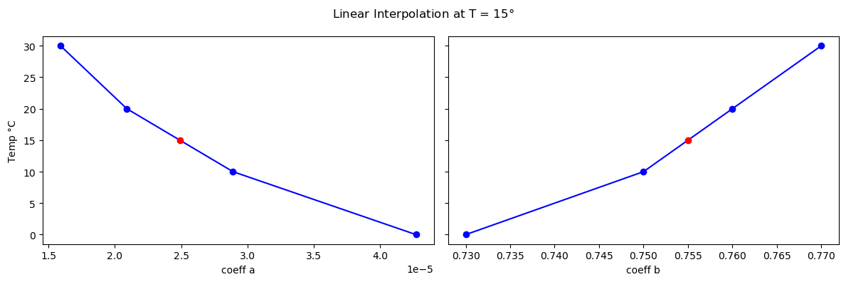
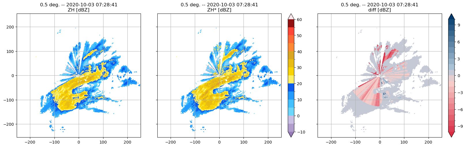
Partial Beam Blockage correction#
The partial beam blockage is corrected using the method proposed by Diederich, M. et al (2015).
temp = 15
rzhah = tp.attc.r_att_refl.Attn_Refl_Relation(rdata)
rzhah.ah_zh(rattc.vars, rband='C', zh_upper_lim=55, temp=temp, copy_ofr=True,
            data2correct=rattc.vars, plot_method=True)
rattc.vars['ZH* [dBZ]'] = rzhah.vars['ZH [dBZ]']
The plot_ppidiff function is useful to visualise the results of the PBB correction:
tp.datavis.rad_display.plot_ppidiff(rdata.georef, rdata.params, rattc.vars,
                                        rattc.vars, var2plot1='ZH [dBZ]',
                                        var2plot2='ZH* [dBZ]')
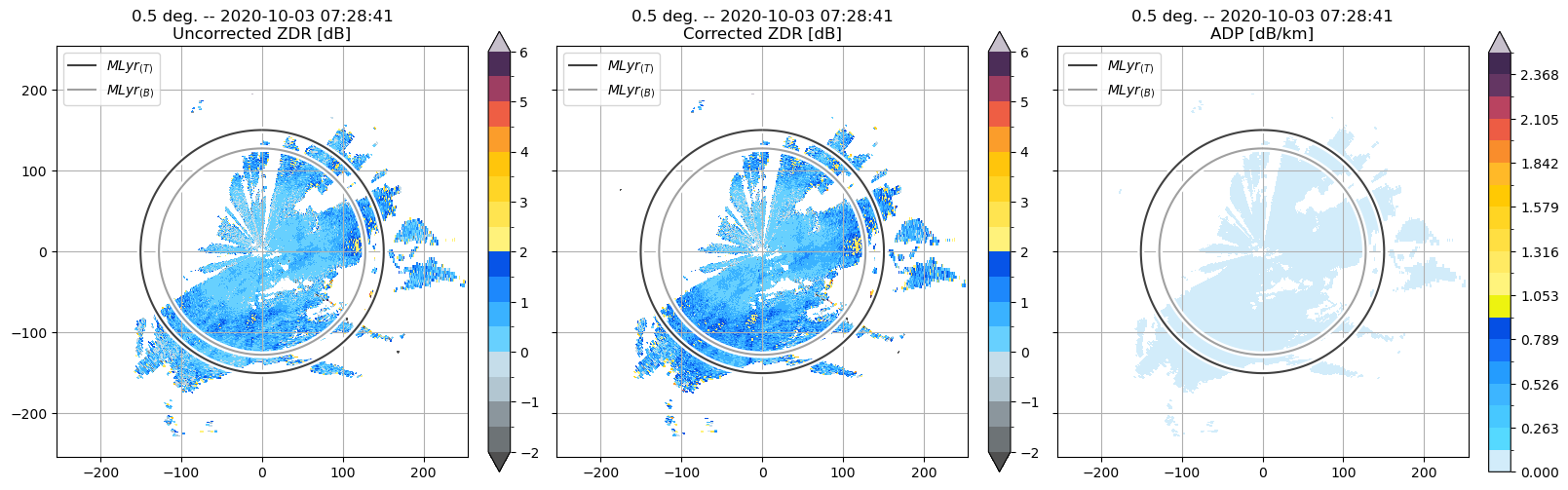
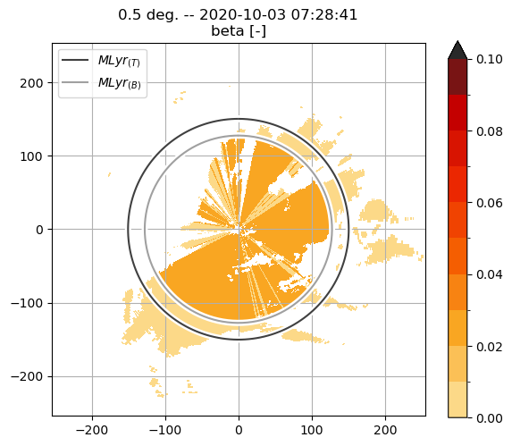
ZDR attenuation correction#
The zdr_correction function requires the outputs of the $Z_H$ attenuation correction (i.e., $\alpha, A_h$) to compute the specific differential attenuation,
rattc.zdr_correction(rdata.georef, rdata.params, rozdr.vars, rattc.vars,
                     rnme.nme_classif['classif [EC]'], mlyr=rmlyr, rhv_thld=0.985,
                     minbins=9, mov_avrgf_len=5, p2avrf=3,
                     plot_method=True)
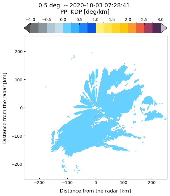
$K_{DP}$ computation#
$K_{DP}$ is an output of the rattc.zh_correction function!
tp.datavis.rad_display.plot_ppi(rdata.georef, rdata.params, rattc.vars,
                                 var2plot='KDP [deg/km]',
                                 vars_bounds={'KDP [deg/km]': (-1, 3, 17)})
Quantitative Precipitation estimation#
We use the RadarQPE class to initialise a radar QPE object.
This class contains several rain estimators, and the coefficients used in each algorithm can be modified by the user depending on the radar frequency or the rainfall regime.
rqpe = tp.qpe.qpe_algs.RadarQPE(rdata)

rqpe.z_to_r(rattc.vars['ZH* [dBZ]'], a=200, b=1.6, mlyr=rmlyr,
            beam_height=rdata.georef['beam_height [km]'])
rqpe.ah_to_r(rattc.vars['AH [dB/km]'], mlyr=rmlyr,
             beam_height=rdata.georef['beam_height [km]'])
rqpe.z_zdr_to_r(rattc.vars['ZH [dBZ]'], rattc.vars['ZDR [dB]'], mlyr=rmlyr,
                beam_height=rdata.georef['beam_height [km]'])
rqpe.kdp_zdr_to_r(rattc.vars['KDP [deg/km]'], rattc.vars['ZDR [dB]'], mlyr=rmlyr,
                  beam_height=rdata.georef['beam_height [km]'])
help(rqpe.ah_to_r)
Help on method ah_to_r in module towerpy.qpe.qpe_algs:

ah_to_r(ah, rband='C', temp=20.0, a=None, b=None, mlyr=None, beam_height=None) method of towerpy.qpe.qpe_algs.RadarQPE instance
    Compute rain rates using the :math:`R(A_{H})` estimator [Eq.1]_.

    Parameters
    ----------
    ah : float or array
        Floats that corresponds to the specific attenuation, in dB/km.
    rband: str
        Frequency band according to the wavelength of the radar.
        The string has to be one of 'S', 'C' or 'X'. The default is 'C'.
    temp: float
        Temperature, in :math:`^{\circ}C`, used to derive the coefficients
        a, b according to [1]_. The default is 20.
    a, b : floats
        Override the computed coefficients of the :math:`R(A_{H})`
        relationship. The default are None.
    mlyr : MeltingLayer Class, optional
        Melting layer class containing the top of the melting layer, (i.e.,
        the melting level) and its thickness. Only gates below the melting
        layer bottom (i.e. the rain region below the melting layer) are
        included in the computation; ml_top and ml_thickness can be either
        a single value (float, int), or an array (or list) of values
        corresponding to each azimuth angle of the scan. If None, the
        rainfall estimator is applied to the whole PPI scan.
    beam_height : array, optional
        Height of the centre of the radar beam, in km.

    Returns
    -------
    R : dict
        Computed rain rates, in mm/h.

    Math
    ----
    .. [Eq.1]
    .. math::  R = aA_H^b
    where R in mm/h, AH in dB/km

    Notes
    -----
    Standard values according to [1]_.

    References
    ----------
    .. [1] Ryzhkov, A., Diederich, M., Zhang, P., & Simmer, C. (2014).
        "Potential Utilization of Specific Attenuation for Rainfall
        Estimation, Mitigation of Partial Beam Blockage, and Radar
        Networking" Journal of Atmospheric and Oceanic Technology, 31(3),
        599-619. https://doi.org/10.1175/JTECH-D-13-00038.1
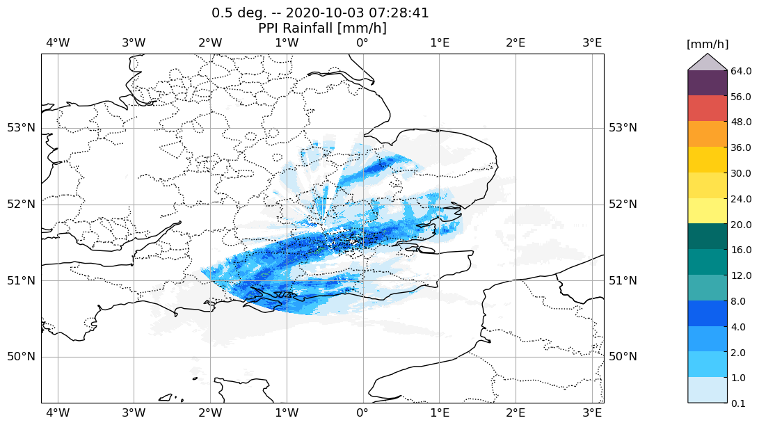
We use the plot_ppi function to display the rain product on a map with a projection corresponding to the location of the radar.
# Plot the radar data in a map
tp.datavis.rad_display.plot_ppi(rdata.georef, rdata.params, rqpe.r_z,
                                data_proj=ccrs.OSGB(approx=False),
                                cpy_feats={'status': True}, fig_size = (12, 6))
©Natural Earth; license: public domain
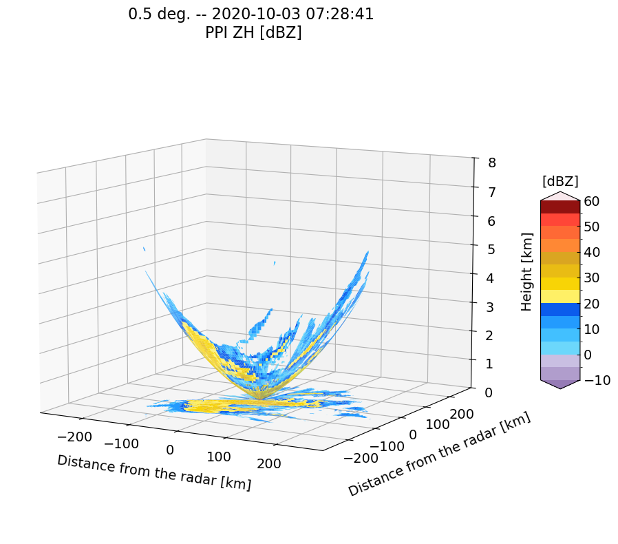
Finally, we use other functions within the datavis module to explore the radar data.
# Plot cone coverage
tp.datavis.rad_display.plot_cone_coverage(rdata.georef, rdata.params,
                                          rsnr.vars)
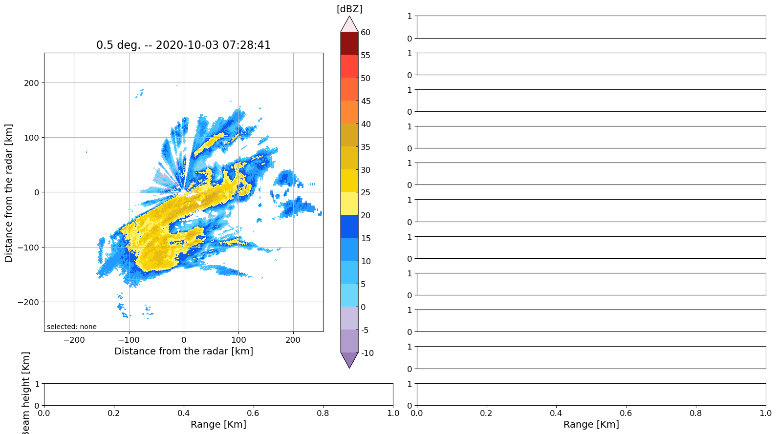
The rad_interactive module#
This module helps explore the PPI scans. For instance, the user can store the coordinates of the current position of the mouse pointer by pressing a number (0-9). This is useful for classifying pixels, e.g. 0 for meteorological echoes, 3 for noise and 5 for non-meteorological ones, in accordance with the clutter_id function.
# Plot an interactive PPI explorer
tp.datavis.rad_interactive.ppi_base(rdata.georef, rdata.params, rattc.vars)
ppiexplorer = tp.datavis.rad_interactive.PPI_Int()
# %%
# ppiexplorer.savearray2binfile(file_name=fname, dir2save='/fdir2/')
 ============================================================
  Right-click on a pixel within the PPI to select its
  azimuth or use the n and m keys to browse through the next
  and previous azimuth.
  Radial profiles of polarimetric variables will be shown at
  the axes on the right.
  Press a number (0-9) to store the coordinates and value
  of the current position of the mouse pointer.
  These coordinate can be retrieved at
  ppiexplorer.clickcoords
 =============================================================
ppiexplorer.clickcoords
[]
References#
V. N. Bringi, T. D. Keenan and V. Chandrasekar, “Correcting C-band radar reflectivity and differential reflectivity data for rain attenuation: a self-consistent method with constraints,” in IEEE Transactions on Geoscience and Remote Sensing, vol. 39, no. 9, pp. 1906-1915, Sept. 2001, https://doi.org/10.1109/36.951081
Diederich, M., Ryzhkov, A., Simmer, C., Zhang, P., & Trömel, S. (2015). Use of Specific Attenuation for Rainfall Measurement at X-Band Radar Wavelengths. Part I: Radar Calibration and Partial Beam Blockage Estimation. Journal of Hydrometeorology, 16(2), 487-502. https://doi.org/10.1175/JHM-D-14-0066.1
Met Office (2003): Met Office Rain Radar Data from the NIMROD System. NCAS British Atmospheric Data Centre, 2022. http://catalogue.ceda.ac.uk/uuid/82adec1f896af6169112d09cc1174499
Rico-Ramirez, M. A., & Cluckie, I. D. (2008). Classification of ground clutter and anomalous propagation using dual-polarization weather radar. IEEE Transactions on Geoscience and Remote Sensing, 46(7), 1892-1904. https://doi.org/10.1109/TGRS.2008.916979
Rico-Ramirez, M. A. (2012) “Adaptive Attenuation Correction Techniques for C-Band Polarimetric Weather Radars,” in IEEE Transactions on Geoscience and Remote Sensing, vol. 50, no. 12, pp. 5061-5071, Dec. 2012. https://doi.org/10.1109/TGRS.2012.2195228